What is transfer learning? How it works, with examples

Transfer learning: what is it?

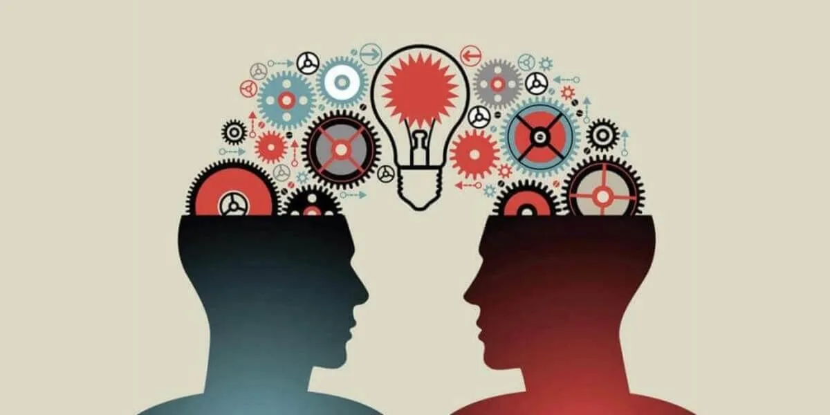
In transfer learning, the knowledge of an already trained machine learning model is applied to a different but related problem. For example, if you have trained a simple classifier to predict whether a picture contains a backpack, you can use the knowledge the model gained during training to recognize other objects, such as sunglasses. We use what was learned in one task to improve generalization in another: we transfer the knowledge the network learned in task A to a new task B.

The general idea is to take what a model learned from a task with plenty of labeled training data and apply it to a new task where data is scarce. Instead of starting the learning process from scratch, you start from the patterns the model learned while solving the related task.

Researchers describe this with four terms: a source domain and source task, where the model was trained, and a target domain and target task, where you want it to work. A domain is the kind of data, such as photos from the web or chest X-rays; a task is what the model predicts from it, such as the object in the photo or signs of pneumonia. Sinno Jialin Pan and Qiang Yang set out this vocabulary in their 2010 survey in IEEE Transactions on Knowledge and Data Engineering, a widely cited reference on the subject.

Transfer learning is not exactly a single Machine Learning technique. It is better seen as a design methodology within machine learning, and it is not tied to one branch of it. It became popular together with neural networks, because they need huge amounts of data and computing power, and transfer learning lets that cost be paid once and reused many times.

The term is older than computers. In psychology, transfer of learning means that practice in one activity changes how well you perform another. Edward Thorndike and Robert Woodworth tested the idea in a series of papers in Psychological Review in 1901 and concluded that practice carries over only where the two tasks share identical elements. Machine learning works on the same intuition: a model transfers well when the source and target tasks share structure.

An example of transfer learning

The most common example comes from computer vision. A network such as ResNet or Inception is first trained on ImageNet, whose standard training set holds about 1.28 million photos in 1,000 categories. That network already knows how to see edges, textures and object parts. A team with a few thousand photos of its own products, crops or machine parts can reuse it and train only the final layers.

A well-documented case comes from medicine. In 2017 a Stanford team published in Nature a skin cancer classifier built exactly this way. They took Google’s Inception v3 network, pretrained on the 1.28 million ImageNet images, removed its final classification layer and retrained it on 129,450 clinical images covering 2,032 diseases. Tested on biopsy-proven images against 21 board-certified dermatologists, it performed on par with all of them in two tasks: telling carcinomas from benign growths, and melanomas from benign moles. The authors name the procedure transfer learning and call it the optimal choice for the amount of data they had.

Other everyday examples follow the same pattern: a speech recognizer trained on clean English adapted to a call center’s vocabulary, a sentiment model trained on movie reviews applied to product reviews, or a control policy trained in simulation moved to a real robot. Language models, covered below, use it at the largest scale of all.

How transfer learning works

In image recognition, neural networks usually learn to detect edges in the first layers, shapes in the middle layers and task-specific features in the last layers. With transfer learning you keep the first and middle layers and retrain only the last ones. That way the model still benefits from the labeled data of the task it was originally trained on.

This is more than an intuition. In 2014 Jason Yosinski, Jeff Clune, Yoshua Bengio and Hod Lipson measured it: the first layer of an image network learns similar filters, resembling Gabor filters and color blobs, whatever the dataset, and features turn from general to specific towards the last layer. They also found that transferability falls as the source and target tasks grow apart, and that starting from transferred features improved generalization even after fine-tuning on the new dataset.

In transfer learning, we try to carry as much knowledge as possible from the previous task to the new one. This knowledge can take different forms depending on the problem and the data: learned features, the weights of whole layers, or the way a model is composed, which makes new objects easier to identify. In practice, the workflow looks like this:

• Pick a pretrained model whose original data is close to yours: an ImageNet network for photos, a language model for text, a model trained on medical images for scans.
• Remove the output layer (the head) that made predictions for the old task and add a new one sized for your classes or values.
• Freeze the pretrained layers so their weights do not change, and train only the new head on your data.
• If you have enough data, unfreeze some of the later layers and keep training with a smaller learning rate, so the useful features are adjusted rather than overwritten.
• Evaluate on data the model has not seen and compare with a model trained from scratch. If the pretrained start does not win, the source model was the wrong one.

Frameworks reduce this to a few lines of code. If the original model was trained using TensorFlow, you can simply restore it and re-create some layers for your task. Keras Applications, PyTorch’s torchvision and the Hugging Face Hub publish pretrained weights ready to download.

Fine-tuning vs feature extraction

The two ways of reusing a model differ in what you allow to change. In feature extraction the pretrained network stays frozen and works as a fixed encoder: it turns each image or text into a vector of features, and only a small new classifier learns from your labels. In fine-tuning you continue training some or all of the pretrained weights on the new data, with a smaller learning rate than the new layers get, because the pretrained weights are already good and should not be distorted too quickly.

Fine-tuning is therefore one way of doing transfer learning, not a separate method. Transfer learning is the broad idea of reusing what a model learned; fine-tuning is the step that adapts its weights to the new task. A common recipe combines both: train the new head with the base frozen first, then unfreeze the top layers and fine-tune them gently.

Stanford’s CS231n course notes give a simple rule for choosing, based on how much labeled data you have and how close it is to the source data:

• Small dataset, similar to the original: train only a linear classifier on the network’s features. Fine-tuning risks overfitting.
• Large dataset, similar to the original: fine-tune the whole network.
• Small dataset, very different from the original: train a linear classifier, but on features from an earlier layer, which are more generic than the top ones.
• Large dataset, very different from the original: you could train from scratch, but initializing with pretrained weights is very often still better.

Types of transfer learning

Pan and Yang’s survey sorts transfer learning by where the labels are:

• Inductive transfer learning: the target task differs from the source task, and you have some labeled target data. Fine-tuning an ImageNet classifier to recognize product defects is inductive.
• Transductive transfer learning: the task stays the same, the domain changes, and labels exist only in the source domain. A spam filter trained on English emails and adapted to French ones is a typical example; most domain adaptation methods belong here.
• Unsupervised transfer learning: neither domain has labels, and the target task is something like clustering or dimensionality reduction.

Two related ideas often appear next to these. Few-shot learning adapts a model to a new class from a handful of examples, and zero-shot learning handles classes the model never saw in training by relying on descriptions or relations it already knows. Both work best on top of large pretrained models.

Transfer learning in language models

Since this post was first written in 2018, transfer learning has moved to the center of AI. That same year, ULMFiT by Jeremy Howard and Sebastian Ruder showed that a language model pretrained on general text and then fine-tuned for classification, with only 100 labeled examples, matched the performance of training from scratch on 100 times more data. In October 2018 Google’s BERT made the recipe standard: one model pretrained on unlabeled text, fine-tuned with just one additional output layer, set new records on eleven language tasks.

In 2021 a Stanford group coined the term foundation models for models trained on broad data at scale and adapted to many downstream tasks, and noted that they rest on standard deep learning and transfer learning. Today’s large language models are built this way: pretrained once on huge amounts of text, then fine-tuned for instructions, chat or a specialist domain. OpenAI’s InstructGPT (2022) shows how much the second stage matters. GPT-3 was fine-tuned on human-written demonstrations and then with reinforcement learning from human feedback, and people preferred the answers of the 1.3 billion parameter fine-tuned model to those of the original 175 billion parameter GPT-3.

Fine-tuning a model with billions of parameters is expensive, so parameter-efficient methods became common. The best known, LoRA (Microsoft, 2021), freezes the pretrained weights and trains small added matrices instead. Compared with fully fine-tuning GPT-3 175B, its authors report 10,000 times fewer trainable parameters and three times less GPU memory. One step further, GPT-3 itself showed in 2020 that a large model can pick up a new task from a few examples written into the prompt, without any change to its weights.

Benefits and limits of transfer learning

Using transfer learning has many advantages. The main ones are that you save training time, your neural network performs better in most cases, and you do not need a lot of data. You can build a solid machine learning model with relatively little training data because the model is already pretrained. This is especially valuable for natural language processing (NLP), because creating large labeled datasets requires expert knowledge.

It is difficult to formulate rules that apply to all of machine learning. You usually use transfer learning when you do not have enough labeled data to train a network from scratch and there is already a network pretrained on a similar task, usually on huge amounts of data. Another case where it fits is when task A and task B have the same kind of input data.

Note that transfer learning works only if the features learned in the first task are generic, which means they are also useful in other, related tasks. When they are not, you meet its main risks:

• Negative transfer: the pretrained start makes results worse than training from scratch, typically when the source and target data have little in common.
• Domain shift: the data looks similar but is distributed differently, such as daylight photos in training and night shots in production. Accuracy drops quietly unless you test on real target data.
• Inherited bias and errors: whatever the pretrained model learned, including skewed data, comes along into the new model.
• Licenses and size: pretrained weights come with licenses that may restrict commercial use, and large models need serious hardware to fine-tune and to run.

Industrial inspection shows both sides. Defects are rare, so a team may have thousands of images of good products and a few dozen of bad ones, a problem known as unbalanced classification. A pretrained network helps the model learn from those few examples, but it still has to be validated on the plant’s own images, whether the task is spotting scratches on metal or finding contaminants on X-ray images of food.